
Introduction
Nvidia has gained a lot of popularity recently, especially with the bloom in artificial intelligence. They have revolutionized the way the powers of their GPUs can be harvested to perform complex tasks in no time. They’ve done so with the introduction of the CUDA Programming Model, first launched in 2006 with the Nvidia GeForce 8800 GTX (built on the G80 architecture).
This blog will familiarize you with the basics of CUDA and get you started on implementing it to solve general problems.
What is a Programming Model?
We must understand what a programming model means before understanding the CUDA programming model.
A programming model defines how the programmer interacts with the hardware, structures their code, and how the data flows.
One example of this concept is the kitchen: The chief chef is given a recipe card (our model) that includes step-by-step instructions in it. The chef executes it one by one.
Following this concept, it divides into two sub-categories:
1. Sequential Model
This model is probably the most common one that most programmers use. Here, the instructions are executed step by step in order just like the chef example given above.
2. Parrallel Programming Model
This model allows many instructions to be executed side by side in parallel. This means no instructions wait for the other. Following our kitchen example, this model allocates many chefs. However, we must change the way we structure our instructions. In this case, instead of handing them a simple step-by-step strategy, each chef will be given their own task.
For example, each chef grabs an onion from the workbench and chops it on their respective counters simultaneously.
How does CUDA Relate?
Traditionally, GPUs were only used for accelerating 3D graphics for games or applications with their intense compute power. They had a large number of cores as opposed to the limited number of cores on the CPU. This allowed rendering frames super fast at many frames per second.
However, with the introduction of the CUDA programming model, Nvidia revolutionized the way these GPUs could be used to accelerate code execution. Their model allowed programmers to harness the power of CUDA cores to allow parallel execution of their code.
The main advantage of this was that large tasks such as matrix multiplication would take milliseconds on the GPU as opposed to seconds on the CPU.
Understanding the Hardware of GPUs
The CPU
Unlike CPUs, GPUs are very different. Most CPUs consist of cores and threads. For example, an Intel CPU might have 4 cores but 8 threads. (These threads are achieved by Intel’s hyper-threading technology or simultaneous multi-threading in AMD). The structure might look something like this:
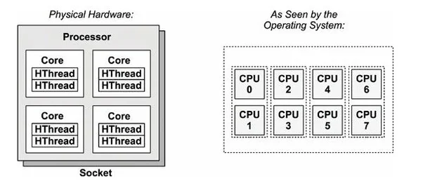 Source of Image: here
Each core exposes two logical processors to the operating system. Each logical core can perform a task. However, only one will execute at a time. For example, if on core 1, thread 1 is waiting for a result to be computed, a task can be executed on thread 2, allowing for minimum latency.
The GPU
Unlike a CPU, a GPU consists of streaming multiprocessors.
The analogy can be understood as follows:
Imagine the CPU is a single master chef in a large kitchen. It has all of its ingredients available right by in its local storage (cache). If the chef needs an ingredient that isn’t in their cache, they might tell their assistant to get it from the storage, while the chef will quickly adopt another task for maximum efficiency.
However, imagine the GPU as a line of workers by the conveyer belt in a factory. None of them are experts at their tasks, but they are able to execute the same processing/task on different variants of items. Same goes for code. If the assembly line has to wait for the new batch of items to arrive, it will quickly switch the entire line to work on a different problem.
Let’s look at the diagram below:
 Source: here
(This may look complicated, but just understand the basic structure for now and ignore the cache and stuff mentioned.)
Organizing Code into Threads and Blocks
Now that we are familiar with the basic structure of the GPU, it is important to understand that we must completely alter the way we approach programming on them. We must structure our code according to the hardware so we utilize the full potential of the GPU with maximum efficiency.
The code that runs on the GPU is called a kernel. and executing that code is referred to as “launching the kernel.”
1. Threads
A thread is the smallest unit of execution in CUDA. Using the same factory example for GPUs from above, a thread is like a worker that is on the factory line. It executes our kernel on a specific piece of data.
2. Blocks
Following threads, a block is a group of threads that is assigned to a specific streaming multiprocessor.
A block can vary in size (e.g., up to 1024 threads) that execute on the same streaming multiprocessor.
Advantages of Grouping Threads into Blocks
1. Scalability
While the CUDA programming model applies to all supported GPUs, many GPUs differ in hardware in terms of their streaming multiprocessor count. However, blocks are completely independent of the hardware.
For example, a GPU with 4 streaming multiprocessors will run 4 blocks at a time, while a GPU with 100 streaming multiprocessors can run 100 blocks at a time.
2. Fast Memory Access
Threads on the same block can access a space of memory inside the streaming multiprocessor called “Shared Memory.” This memory is managed by the programmer, and since it is inside the streaming multiprocessor itself, it is super fast to read.
This way, instead of refetching data from the slower memory, the needed data is kept in shared memory, hence reducing latency.
3. Optimal Resource Allocation
The resources used by the blocks can vary, and if the resources used by a block are low, the streaming multiprocessor loads multiple blocks concurrently to keep the hardware units fully utilized.
Memory Hierachy
Before we move on to implementing and writing our first CUDA program, we must understand the layout of registers and memory in a GPU.
Look at the diagram below:
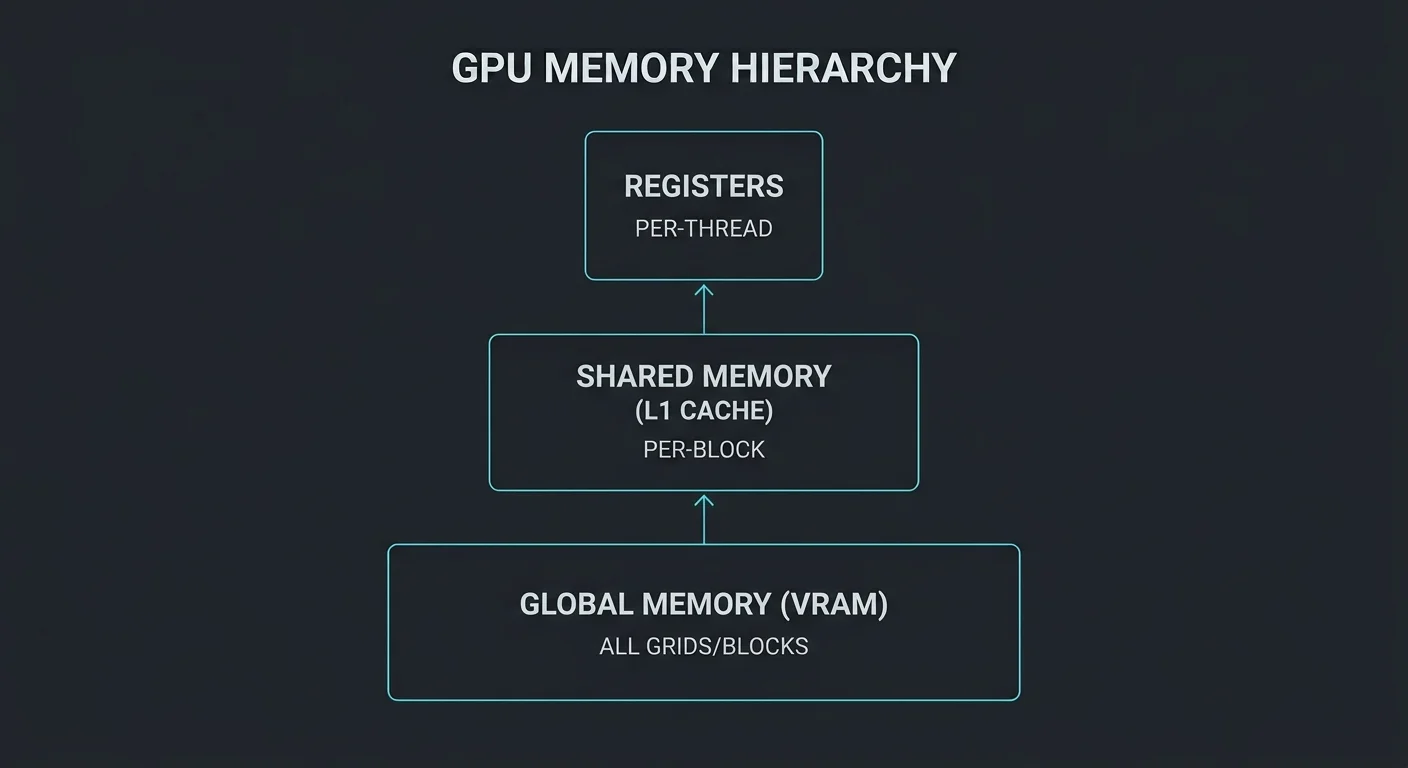
This hierarchy shows that registers are the fastest available memory. However, they have a finite size and are generally used for storing variables. If the data exceeds the size of the registers, it spills it to the slower local memory (VRAM). Each thread gets its own register file.
After registers, shared memory is the second-fastest memory available to all threads in the same block. If the data size exceeds the size of shared memory, the kernel needs to store its data in the slower DRAM by explicitly allocating from it.
Implementing CUDA
Linear algebra has become highly relevant with the growing applications of AI. As during my current semester 3, I am studying this course, to implement the concepts we just learned, I’ll be demonstrating the code via the most common kernel written for the GPUs: matrix multiplication.
We will first implement it by solving it via the CPU and then by solving the same problem on my GPU (RTX 3060 Mobile).
Setting Up NVCC
NOTE: This will only work for systems with CUDA-supported Nvidia GPUs. However, the CPU demonstration below can be implemented in traditional C++ with G++ as well.
We will be writing our code in the .cu format, which is basically C++ with Nvidia’s extensions.
The compiler used to compile .cu files is NVCC (Nvidia CUDA Compiler).
To Install it, simply run the below commands:
- For Arch-based systems:
sudo pacman -Sy cuda nvidia-utils
- For debain-based systems:
sudo apt install cuda-toolkit
Read this guide for other operating systems: here.
Implementing Matrix Multiplication on CPU
The logic is simple: we are given matrices A and B. Multiplication will result in matrix C. To do this, we will calculate each entry of the resultant matrix one by one.
Let’s look at the function below:
// Multiplies two matrixes A, B and stores it in matrix C.
void multiplyMatrix(float *matrixA, float *matrixB, float *resultMatrix, int colA, int rowsA, int colB)
{

    // Loop through rows of A
    for (int i = 0; i < rowsA; i++)
    {

        // Loop through columns of B
        for (int j = 0; j < colB; j++)
        {
            float product = 0;

            // Loop through row entries of A
            for (int k = 0; k < colA; k++)
            {
                int indexA = (i * colA + k);
                int indexB = (k * colB + j); // k*colB jumps to respective row for that entry. basically the kth entry in column.

                product += matrixA[indexA] * matrixB[indexB]; // Add to product
            }

            int resultIndex = i * colB + j; // i is the A's current row. multiplying it with colB jumps it to relevant row and its relevant column j.

            resultMatrix[resultIndex] = product;
        }
    }
}
The above function simply uses nested loops to calculate the resultant matrix. I’ve added comments to help you understand what each line does.
Our main function will look something like this:
int main()
{

    int rowsA = 1024;
    int colA = 1024;

    int rowsB = 1024;
    int colB = 1024;

    int sizeA = rowsA * colA;
    int sizeB = rowsB * colB;
    int sizeResult = rowsA * colB;

    float *matrixA = new float[sizeA];
    float *matrixB = new float[sizeB];
    float *resultMatrix = new float[sizeResult];

    // Initialize matrixA with multiples of 10 all the way through

    int temp = 10;
    for (int i = 0; i < sizeA; i++)
    {
        matrixA[i] = temp;
        temp += 10;
    }

    temp = 0;
    for (int i = 0; i < sizeB; i++)
    {
        matrixB[i] = temp;
        temp += 10;
    }

    auto start = std::chrono::high_resolution_clock::now();

    multiplyMatrix(matrixA, matrixB, resultMatrix, colA, rowsA, colB);

    auto end = std::chrono::high_resolution_clock::now();

    chrono::duration<double, std::milli> durationMs = end - start;
    std::cout << "Execution Time: " << durationMs.count() << " ms\n";

    // NO MEM LEAKS PLIJ!!!!!!!
    delete[] matrixA;
    delete[] matrixB;
    delete[] resultMatrix;

    return 0;
}
We simply allocate a matrix of 1024 x 1024, initialize the values with multiples of 10 with a for loop, and store the result in our resultant matrix. chrono is being used here to calculate the time taken by the calculation.
We can compile this code by running:
nvcc cpu_matrix.cu -o cpu_matrix
./cpu_matrix # Might be different on Windows
The resultant output is:
Execution Time: 3075.03 ms
The calculation took a whopping 3 seconds!
The loop iterated through each row and column one by one, and hence, the time complexity scaled intensively.
Implementing Matrix Multiplication on GPU
Remember how I said we must change the way we think and the way we structure our code?
It finally comes into play. Instead of iterating through columns and rows one by one, we assign each thread to their own respective element.
We must first understand how each thread is structured in the CUDA programming model.
Look at the diagram below:

Threads are arranged in this grid. We can specify threads per block and blocks per grid.
Look at our kernel below:
// Multiplies two matrixes A, B and stores it in matrix C.
__global__ void multiplyMatrixKernel(float *matrixA, float *matrixB, float *resultMatrix, int colA, int rowsA, int colB)
{

    int row = blockIdx.y * blockDim.y + threadIdx.y;
    int column = blockIdx.x * blockDim.x + threadIdx.x;

    if (row < rowsA && column < colB)
    {

        float product = 0;

        // Loop through row entries of A
        for (int k = 0; k < colA; k++)
        {
            int indexA = (row * colA + k);
            int indexB = (k * colB + column); // k*colB jumps to respective row for that entry. basically the kth entry in column.

            product += matrixA[indexA] * matrixB[indexB]; // Add to product
        }

        int resultIndex = row * colB + column; // i is the A's current row. multiplying it with colB jumps it to relevant row and its relevant column j.

        resultMatrix[resultIndex] = product;
    }
}
Notice the __global__ operand before the return type of our kernel?
This specifies that this function will be executed on our GPU.
Each row and column’s index is calculated by the below formulas:
int row = blockIdx.y * blockDim.y + threadIdx.y;int column = blockIdx.x * blockDim.x + threadIdx.x;blockIdx.y=> the vertical index of our blockblockIdx.x=> the horizontal index of our blockthreadIdx.y=> the row position of the thread.threadIdx.x=> the column position of the thread.
The line blockIdx.y * blockDim.y and blockIdx.x * blockDim.x jump across to the first entry of our row and column. threadIdx then acts as the offset to reach our element.
Loops have been removed since each row and column is assigned its own thread.
Let’s have a look at our main code now:
int main()
{

    int rowsA = 1024;
    int colA = 1024;

    int rowsB = 1024;
    int colB = 1024;

    size_t sizeA = rowsA * colA;
    size_t sizeB = rowsB * colB;
    size_t sizeResult = rowsA * colB;

    float *host_matrixA = new float[sizeA];
    float *host_matrixB = new float[sizeB];
    float *host_resultMatrix = new float[sizeResult];

    float *device_matrixA, *device_matrixB, *device_resultMatrix;
    cudaMalloc(&device_matrixA, sizeA * sizeof(float));
    cudaMalloc(&device_matrixB, sizeB * sizeof(float));
    cudaMalloc(&device_resultMatrix, sizeResult * sizeof(float));

    // Initialize matrixA with multiples of 10 all the way through

    int temp = 10;
    for (int i = 0; i < sizeA; i++)
    {
        host_matrixA[i] = temp;
        temp += 10;
    }

    temp = 0;
    for (int i = 0; i < sizeB; i++)
    {
        host_matrixB[i] = temp;
        temp += 10;
    }

    cudaMemcpy(device_matrixA, host_matrixA, sizeA * sizeof(float), cudaMemcpyHostToDevice);
    cudaMemcpy(device_matrixB, host_matrixB, sizeB * sizeof(float), cudaMemcpyHostToDevice);


    dim3 threadsPerBlock(32, 32);

    dim3 blocksPerGrid((colB + threadsPerBlock.x - 1) / threadsPerBlock.x,
                       (rowsA + threadsPerBlock.y - 1) / threadsPerBlock.y);

    auto start = std::chrono::high_resolution_clock::now();

    multiplyMatrixKernel<<<blocksPerGrid, threadsPerBlock>>>(device_matrixA, device_matrixB, device_resultMatrix, colA, rowsA, colB);

    cudaDeviceSynchronize();

    auto end = std::chrono::high_resolution_clock::now();

    chrono::duration<double, std::milli> durationMs = end - start;

    cudaMemcpy(host_resultMatrix, device_resultMatrix, sizeResult * sizeof(float), cudaMemcpyDeviceToHost);

    std::cout << "Execution Time: " << durationMs.count() << " ms\n";

    // NO MEM LEAKS PLIJ!!!!!!!

    cudaFree(device_matrixA);
    cudaFree(device_matrixB);
    cudaFree(device_resultMatrix);


    delete[] host_matrixA;
    delete[] host_matrixB;
    delete[] host_resultMatrix;


    return 0;
}
Few things have changed in the above snippet:
- We are declaring new pointers called
device_xxxxwhere xxxx is our matrix. - We are calling
CudaMallocfor each device pointer that is allocating the space for us inside VRAM. - We are copying the data from host to device memory using
CudaMemcpybefore performing operations on it. - using either the
cudaMemcpyHostToDeviceorcudaMemcpyDeviceToHost. - We are declaring a dim3 object called
threadsPerBlockinitialized with values 32x32. - We are declaring a dim3 object called
blocksPerGridinitialized with a formula. - We launch the kernel with some specific configurations using
<<>> cudaDeviceSynchronizeis being called- Allocated device memory is being deallocated.
Before we continue, we must answer, what is the difference between device memory and host memory?
- Host memory: It is the memory associated with the CPU. This is our primary RAM.
- Device memory: It is the memory associated with the GPU. This is the VRAM, which is faster than our primary RAM.
Now that we understand these two definitions, it makes sense why we perform the cudaMemcpy operations.
We must move our relevant data closer to the GPU before the kernel is launched. So that when it retrieves the needed data, it does not have to repeatedly go to the slower system host memory, which will result in increased latency.
After our operations are done, we must move the calculated result back into the host memory for reading and using it for other purposes.
However, before we continue with other operations, we use cudaDeviceSynchronize() to allow for all the threads to complete their task; only then does the code continue.
The Kernel Configuration
Let’s now talk about the dim3 objects and the configuration specified via <<>>
dim3 is a built-in datatype that allows us to define grids.
For example, dim3 T(32, 32) defines a grid of 32 x 32.
The kernel needs to be passed two operands:
- Threads per block: We define how many threads live inside a single block.
- Blocks per grid: We define how many blocks are needed to cover the entire dataset.
You might’ve noticed this formula for blocksPerGrid:
(colB + threadsPerBlock.x - 1) / threadsPerBlock.x and rowsA + threadsPerBlock.y - 1) / threadsPerBlock.y
This is actually a standard formula for ceiling division. It ensures no entry is left out.
For example, let’s say we have 1000 matrix rows / columns and a block size of 32:
using standard division:
1000 / 32 = 31
31 x 32 = 992 <= Index 992 up till 999 is never evaluated.
with ceiling division:
1000 / 32 = 32
32 x 32 = 1024 <= Guaranteed 100% coverage
Now let’s look at our output of the GPU example:
Execution Time: 3.34882 ms
3 MILLISECONDS! That is a drastic decrease in execution time.
Summary
CUDA is a revolutionary technology that has not only provided a base to perform large calculations but is also being used today to run AI infrastructure across various domains. It turned existing computational hardware used for 3D acceleration into a tool for parallel computing!